A Deep Dive Into The Mathematics Of Pauli Matrices

Understand the mathematical properties of Pauli matrices to use them like a pro in Quantum computing.

A 1929 photograph of Wolfgang Pauli, a theoretical physicist and pioneer of quantum mechanics, best known for formulating the Pauli exclusion principle and receiving the 1945 Nobel Prize in Physics for his contributions to the understanding of atomic structure (Source)

Pauli matrices are a set of three matrices that are absolutely essential in Quantum computing.

These matrices, termed Pauli-X (σ(x) or σ(1)), Pauli-Y (σ(y) or σ(2)), and Pauli-Z (σ(z) or σ(3)), are shown below:

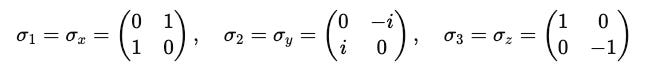
They are named after the phenomenal physicist Wolfgang Pauli, who won the 1945 Nobel Prize in Physics for discovering the Pauli exclusion principle.

In this lesson, we discuss some of the elegant mathematical properties that these matrices possess that make them so useful in Quantum computing.

---

Pauli Matrices In A Single Expression

All three of the Pauli matrices can be represented compactly using the following equation:

where:

• j is the Pauli matrix we are referring to (j ∈ {1,2,3})

• δ(i)(j) is the Kronecker delta

---

Pauli Matrices are Hermitian

Each Pauli matrix is a square matrix that is equal to its own conjugate transpose. This means that they are Hermitian matrices.

As an example, Pauli-X, as shown below:

Its complex conjugate is:

The transpose of this term is:

This is overall the same as the Hermitian (†) operation and:

Pauli matrices, being Hermitian, always have real eigenvalues.

Since measurements in physics must yield real values, this makes them suitable for being used as operators corresponding to physical observables, specifically Spin.